Zero-Hitting and Failure of the Martingale Property

For nonnegative local martingales, there is an interesting symmetry between the failure of the martingale property and the possibility of hitting zero, which I will describe now. I will also give a necessary and sufficient condition for solutions to a certain class of stochastic differential equations to hit zero in finite time and, using the aforementioned symmetry, infer a necessary and sufficient condition for the processes to be proper martingales. It is often the case that solutions to SDEs are clearly local martingales, but is hard to tell whether they are proper martingales. So, the martingale condition, given in Theorem 4 below, is a useful result to know. The method described here is relatively new to me, only coming up while preparing the previous post. Applying a hedging argument, it was noted that the failure of the martingale property for solutions to the SDE ${dX=X^c\,dB}$ for ${c>1}$ is related to the fact that, for ${c<1}$ , the process hits zero. This idea extends to all continuous and nonnegative local martingales. The Girsanov transform method applied here is essentially the same as that used by Carlos A. Sin (Complications with stochastic volatility models, Adv. in Appl. Probab. Volume 30, Number 1, 1998, 256-268) and B. Jourdain (Loss of martingality in asset price models with lognormal stochastic volatility, Preprint CERMICS, 2004-267).

Consider nonnegative solutions to the stochastic differential equation

$\displaystyle \setlength\arraycolsep{2pt} \begin{array}{rl} &\displaystyle dX=a(X)X\,dB,\smallskip\\ &\displaystyle X_0=x_0, \end{array}$

(1)

where ${a\colon{\mathbb R}_+\rightarrow{\mathbb R}}$ , B is a Brownian motion and the fixed initial condition ${x_0}$ is strictly positive. The multiplier X in the coefficient of dB ensures that if X ever hits zero then it stays there. By time-change methods, uniqueness in law is guaranteed as long as a is nonzero and ${a^{-2}}$ is locally integrable on ${(0,\infty)}$ . Consider also the following SDE,

$\displaystyle \setlength\arraycolsep{2pt} \begin{array}{rl} &\displaystyle dY=\tilde a(Y)Y\,dB,\smallskip\\ &\displaystyle Y_0=y_0,\smallskip\\ &\displaystyle \tilde a(y) = a(y^{-1}),\ y_0=x_0^{-1} \end{array}$

(2)

Being integrals with respect to Brownian motion, solutions to (1) and (2) are local martingales. It is possible for them to fail to be proper martingales though, and they may or may not hit zero at some time. These possibilities are related by the following result.

Theorem 1 Suppose that (1) and (2) satisfy uniqueness in law. Then, X is a proper martingale if and only if Y never hits zero. Similarly, Y is a proper martingale if and only if X never hits zero.

Continue reading “Zero-Hitting and Failure of the Martingale Property” →

Failure of the Martingale Property

In this post, I give an example of a class of processes which can be expressed as integrals with respect to Brownian motion, but are not themselves martingales. As stochastic integration preserves the local martingale property, such processes are guaranteed to be at least local martingales. However, this is not enough to conclude that they are proper martingales. Whereas constructing examples of local martingales which are not martingales is a relatively straightforward exercise, such examples are often slightly contrived and the martingale property fails for obvious reasons (e.g., double-loss betting strategies). The aim here is to show that the martingale property can fail for very simple stochastic differential equations which are likely to be met in practice, and it is not always obvious when this situation arises.

Consider the following stochastic differential equation

$\displaystyle \setlength\arraycolsep{2pt} \begin{array}{rl} &\displaystyle dX = aX^c\,dB +b X dt,\smallskip\\ &\displaystyle X_0=x, \end{array}$

(1)

for a nonnegative process X. Here, B is a Brownian motion and a,b,c,x are positive constants. This a common SDE appearing, for example, in the constant elasticity of variance model for option pricing. Now consider the following question: what is the expected value of X at time t?

The obvious answer seems to be that ${{\mathbb E}[X_t]=xe^{bt}}$ , based on the idea that X has growth rate b on average. A more detailed argument is to write out (1) in integral form

$\displaystyle X_t=x+\int_0^t\,aX^c\,dB+ \int_0^t bX_s\,ds.$

(2)

The next step is to note that the first integral is with respect to Brownian motion, so has zero expectation. Therefore,

$\displaystyle {\mathbb E}[X_t]=x+\int_0^tb{\mathbb E}[X_s]\,ds.$

This can be differentiated to obtain the ordinary differential equation ${d{\mathbb E}[X_t]/dt=b{\mathbb E}[X_t]}$ , which has the unique solution ${{\mathbb E}[X_t]={\mathbb E}[X_0]e^{bt}}$ .

In fact this argument is false. For ${c\le1}$ there is no problem, and ${{\mathbb E}[X_t]=xe^{bt}}$ as expected. However, for all ${c>1}$ the conclusion is wrong, and the strict inequality ${{\mathbb E}[X_t]<xe^{bt}}$ holds.

The point where the argument above falls apart is the statement that the first integral in (2) has zero expectation. This would indeed follow if it was known that it is a martingale, as is often assumed to be true for stochastic integrals with respect to Brownian motion. However, stochastic integration preserves the local martingale property and not, in general, the martingale property itself. If ${c>1}$ then we have exactly this situation, where only the local martingale property holds. The first integral in (2) is not a proper martingale, and has strictly negative expectation at all positive times. The reason that the martingale property fails here for ${c>1}$ is that the coefficient ${aX^c}$ of dB grows too fast in X.

In this post, I will mainly be concerned with the special case of (1) with a=1 and zero drift.

$\displaystyle \setlength\arraycolsep{2pt} \begin{array}{rl} &\displaystyle dX=X^c\,dB,\smallskip\\ &\displaystyle X_0=x. \end{array}$

(3)

The general form (1) can be reduced to this special case, as I describe below. SDEs (1) and (3) do have unique solutions, as I will prove later. Then, as X is a nonnegative local martingale, if it ever hits zero then it must remain there (0 is an absorbing boundary).

The solution X to (3) has the following properties, which will be proven later in this post.

If ${c\le1}$ then X is a martingale and, for ${c<1}$ , it eventually hits zero with probability one.
If ${c>1}$ then X is a strictly positive local martingale but not a martingale. In fact, the following inequality holds

$\displaystyle {\mathbb E}[X_t\mid\mathcal{F}_s]<X_s$ (4)

(almost surely) for times ${s<t}$ . Furthermore, for any positive constant ${p<2c-1}$ , ${{\mathbb E}[X_t^p]}$ is bounded over ${t\ge0}$ and tends to zero as ${t\rightarrow\infty}$ .

Continue reading “Failure of the Martingale Property” →

Bessel Processes

A random variable ${N=(N^1,\ldots,N^n)}$ has the standard n-dimensional normal distribution if its components ${N^i}$ are independent normal with zero mean and unit variance. A well known fact of such distributions is that they are invariant under rotations, which has the following consequence. The distribution of ${Z\equiv\Vert N+\boldsymbol{\mu}\Vert^2}$ is invariant under rotations of ${\boldsymbol{\mu}\in{\mathbb R}^n}$ and, hence, is fully determined by the values of ${n\in{\mathbb N}}$ and ${\mu=\Vert\boldsymbol{\mu}\Vert^2\in{\mathbb R}_+}$ . This is known as the noncentral chi-square distribution with n degrees of freedom and noncentrality parameter ${\mu}$ , and denoted by ${\chi^2_n(\mu)}$ . The moment generating function can be computed,

$\displaystyle M_Z(\lambda)\equiv{\mathbb E}\left[e^{\lambda Z}\right]=\left(1-2\lambda\right)^{-\frac{n}{2}}\exp\left(\frac{\lambda\mu}{1-2\lambda}\right),$

(1)

which holds for all ${\lambda\in{\mathbb C}}$ with real part bounded above by 1/2.

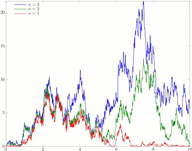
A consequence of this is that the norm ${\Vert B_t\Vert}$ of an n-dimensional Brownian motion B is Markov. More precisely, letting ${\mathcal{F}_t=\sigma(B_s\colon s\le t)}$ be its natural filtration, then ${X\equiv\Vert B\Vert^2}$ has the following property. For times ${s<t}$ , conditional on ${\mathcal{F}_s}$ , ${X_t/(t-s)}$ is distributed as ${\chi^2_n(X_s/(t-s))}$ . This is known as the `n-dimensional’ squared Bessel process, and denoted by ${{\rm BES}^2_n}$ .

A Poisson process sample path — Figure 1: Squared Bessel processes of dimensions n=1,2,3

Alternatively, the process X can be described by a stochastic differential equation (SDE). Applying integration by parts,

$\displaystyle dX = 2\sum_iB^i\,dB^i+\sum_id[B^i].$

(2)

As the standard Brownian motions have quadratic variation ${[B^i]_t=t}$ , the final term on the right-hand-side is equal to ${n\,dt}$ . Also, the covarations ${[B^i,B^j]}$ are zero for ${i\not=j}$ from which it can be seen that

$\displaystyle W_t = \sum_i\int_0^t1_{\{B\not=0\}}\frac{B^i}{\Vert B\Vert}\,dB^i$

is a continuous local martingale with ${[W]_t=t}$ . By Lévy’s characterization, W is a Brownian motion and, substituting this back into (2), the squared Bessel process X solves the SDE

$\displaystyle dX=2\sqrt{X}\,dW+ndt.$

(3)

The standard existence and uniqueness results for stochastic differential equations do not apply here, since ${x\mapsto2\sqrt{x}}$ is not Lipschitz continuous. It is known that (3) does in fact have a unique solution, by the Yamada-Watanabe uniqueness theorem for 1-dimensional SDEs. However, I do not need and will not make use of this fact here. Actually, uniqueness in law follows from the explicit computation of the moment generating function in Theorem 5 below.

Although it is nonsensical to talk of an n-dimensional Brownian motion for non-integer n, Bessel processes can be extended to any real ${n\ge0}$ . This can be done either by specifying its distributions in terms of chi-square distributions or by the SDE (3). In this post I take the first approach, and then show that they are equivalent. Such processes appear in many situations in the theory of stochastic processes, and not just as the norm of Brownian motion. It also provides one of the relatively few interesting examples of stochastic differential equations whose distributions can be explicitly computed.

The ${\chi^2_n(\mu)}$ distribution generalizes to all real ${n\ge0}$ , and can be defined as the unique distribution on ${{\mathbb R}_+}$ with moment generating function given by equation (1). If ${Z_1\sim\chi_m(\mu)}$ and ${Z_2\sim\chi_n(\nu)}$ are independent, then ${Z_1+Z_2}$ has moment generating function ${M_{Z_1}(\lambda)M_{Z_2}(\lambda)}$ and, therefore, has the ${\chi^2_{m+n}(\mu+\nu)}$ distribution. That such distributions do indeed exist can be seen by constructing them. The ${\chi^2_n(0)}$ distribution is a special case of the Gamma distribution and has probability density proportional to ${x^{n/2-1}e^{-x/2}}$ . If ${Z_1,Z_2,\ldots}$ is a sequence of independent random variables with the standard normal distribution and T independently has the Poisson distribution of rate ${\mu/2}$ , then ${\sum_{i=1}^{2T}Z_i^2\sim\chi_0^2(\mu)}$ , which can be seen by computing its moment generating function. Adding an independent ${\chi^2_n(0)}$ random variable Y to this produces the ${\chi^2_n(\mu)}$ variable ${Z\equiv Y+\sum_{i=1}^{2T}Z_i^2}$ .

The definition of squared Bessel processes of any real dimension ${n\ge0}$ is as follows. We work with respect to a filtered probability space ${(\Omega,\mathcal{F},\{\mathcal{F}_t\}_{t\ge0},{\mathbb P})}$ .

Definition 1 A process X is a squared Bessel process of dimension ${n\ge0}$ if it is continuous, adapted and, for any ${s<t}$ , conditional on ${\mathcal{F}_s}$ , ${X_t/(t-s)}$ has the ${\chi^2_n\left(X_s/(t-s)\right)}$ distribution.

Continue reading “Bessel Processes” →

Properties of Feller Processes

In the previous post, the concept of Feller processes was introduced. These are Markov processes whose transition function ${\{P_t\}_{t\ge0}}$ satisfies certain continuity conditions. Many of the standard processes we study satisfy the Feller property, such as standard Brownian motion, Poisson processes, Bessel processes and Lévy processes as well as solutions to many stochastic differential equations. It was shown that all Feller processes admit a cadlag modification. In this post I state and prove some of the other useful properties satisfied by such processes, including the strong Markov property, quasi-left-continuity and right-continuity of the filtration. I also describe the basic properties of the infinitesimal generators. The results in this post are all fairly standard and can be found, for example, in Revuz and Yor (Continuous Martingales and Brownian Motion).

As always, we work with respect to a filtered probability space ${(\Omega,\mathcal{F},\{\mathcal{F}_t\}_{t\ge0},{\mathbb P})}$ . Throughout this post we consider Feller processes X and transition functions ${\{P_t\}_{t\ge0}}$ defined on the lccb (locally compact with a countable base) space E which, taken together with its Borel sigma-algebra, defines a measurable space ${(E,\mathcal{E})}$ .

Recall that the law of a homogeneous Markov process X is described by a transition function ${\{P_t\}_{t\ge0}}$ on some measurable space ${(E,\mathcal{E})}$ . This specifies that the distribution of ${X_t}$ conditional on the history up until an earlier time ${s<t}$ is given by the measure ${P_{t-s}(X_s,\cdot)}$ . Equivalently,

$\displaystyle {\mathbb E}[f(X_t)\mid\mathcal{F}_s]=P_{t-s}f(X_s)$

for any bounded and measurable function ${f\colon E\rightarrow{\mathbb R}}$ . The strong Markov property generalizes this idea to arbitrary stopping times.

Definition 1 Let X be an adapted process and ${\{P_t\}_{t\ge 0}}$ be a transition function.

Then, X satisfies the strong Markov property if, for each stopping time ${\tau}$ , conditioned on ${\tau<\infty}$ the process ${\{X_{\tau+t}\}_{t\ge0}}$ is Markov with the given transition function and with respect to the filtration ${\{\mathcal{F}_{\tau+t}\}_{t\ge0}}$ .

As we see in a moment, Feller processes satisfy the strong Markov property. First, as an example, consider a standard Brownian motion B, and let ${\tau}$ be the first time at which it hits a fixed level ${K>0}$ . The reflection principle states that the process ${\tilde B}$ defined to be equal to B up until time ${\tau}$ and reflected about K afterwards, is also a standard Brownian motion. More precisely,

$\displaystyle \tilde B_t=\begin{cases} B_t,&\textrm{if }t\le\tau,\\ 2K-B_t,&\textrm{if }t\ge\tau, \end{cases}$

is a Brownian motion. This useful idea can be used to determine the distribution of the maximum ${B^*_t=\max_{s\le t}B_s}$ . If ${B^*_t\ge K}$ then either the process itself ends up above K or it hits K and then drops below this level by time t, in which case ${\tilde B_t>K}$ . So, by the reflection principle,

$\displaystyle {\mathbb P}(B^*_t\ge K)={\mathbb P}(B_t\ge K)+{\mathbb P}(\tilde B_t> K)=2{\mathbb P}(B_t\ge K).$

Continue reading “Properties of Feller Processes” →

Feller Processes

The definition of Markov processes, as given in the previous post, is much too general for many applications. However, many of the processes which we study also satisfy the much stronger Feller property. This includes Brownian motion, Poisson processes, Lévy processes and Bessel processes, all of which are considered in these notes. Once it is known that a process is Feller, many useful properties follow such as, the existence of cadlag modifications, the strong Markov property, quasi-left-continuity and right-continuity of the filtration. In this post I give the definition of Feller processes and prove the existence of cadlag modifications, leaving the further properties until the next post.

The definition of Feller processes involves putting continuity constraints on the transition function, for which it is necessary to restrict attention to processes lying in a topological space ${(E,\mathcal{T}_E)}$ . It will be assumed that E is locally compact, Hausdorff, and has a countable base (lccb, for short). Such spaces always possess a countable collection of nonvanishing continuous functions ${f\colon E\rightarrow{\mathbb R}}$ which separate the points of E and which, by Lemma 6 below, helps us construct cadlag modifications. Lccb spaces include many of the topological spaces which we may want to consider, such as ${{\mathbb R}^n}$ , topological manifolds and, indeed, any open or closed subset of another lccb space. Such spaces are always Polish spaces, although the converse does not hold (a Polish space need not be locally compact).

Given a topological space E, ${C_0(E)}$ denotes the continuous real-valued functions vanishing at infinity. That is, ${f\colon E\rightarrow{\mathbb R}}$ is in ${C_0(E)}$ if it is continuous and, for any ${\epsilon>0}$ , the set ${\{x\colon \vert f(x)\vert\ge\epsilon\}}$ is compact. Equivalently, its extension to the one-point compactification ${E^*=E\cup\{\infty\}}$ of E given by ${f(\infty)=0}$ is continuous. The set ${C_0(E)}$ is a Banach space under the uniform norm,

$\displaystyle \Vert f\Vert\equiv\sup_{x\in E}\vert f(x)\vert.$

We can now state the general definition of Feller transition functions and processes. A topological space ${(E,\mathcal{T}_E)}$ is also regarded as a measurable space by equipping it with its Borel sigma algebra ${\mathcal{B}(E)=\sigma(\mathcal{T})}$ , so it makes sense to talk of transition probabilities and functions on E.

Definition 1 Let E be an lccb space. Then, a transition function ${\{P_t\}_{t\ge 0}}$ is Feller if, for all ${f\in C_0(E)}$ ,

${P_tf\in C_0(E)}$ .

${t\mapsto P_tf}$ is continuous with respect to the norm topology on ${C_0(E)}$ .

${P_0f=f}$ .

A Markov process X whose transition function is Feller is a Feller process.

Continue reading “Feller Processes” →

Markov Processes

In these notes, the approach taken to stochastic calculus revolves around stochastic integration and the theory of semimartingales. An alternative starting point would be to consider Markov processes. Although I do not take the second approach, all of the special processes considered in the current section are Markov, so it seems like a good idea to introduce the basic definitions and properties now. In fact, all of the special processes considered (Brownian motion, Poisson processes, Lévy processes, Bessel processes) satisfy the much stronger property of being Feller processes, which I will define in the next post.

Intuitively speaking, a process X is Markov if, given its whole past up until some time s, the future behaviour depends only its state at time s. To make this precise, let us suppose that X takes values in a measurable space ${(E,\mathcal{E})}$ and, to denote the past, let ${\mathcal{F}_t}$ be the sigma-algebra generated by ${\{X_s\colon s\le t\}}$ . The Markov property then says that, for any times ${s\le t}$ and bounded measurable function ${f\colon E\rightarrow{\mathbb R}}$ , the expected value of ${f(X_t)}$ conditional on ${\mathcal{F}_s}$ is a function of ${X_s}$ . Equivalently,

$\displaystyle {\mathbb E}\left[f(X_t)\mid\mathcal{F}_s\right]={\mathbb E}\left[f(X_t)\mid X_s\right]$

(1)

(almost surely). More generally, this idea makes sense with respect to any filtered probability space ${\mathbb{F}=(\Omega,\mathcal{F},\{\mathcal{F}_t\}_{t\ge 0},{\mathbb P})}$ . A process X is Markov with respect to ${\mathbb{F}}$ if it is adapted and (1) holds for times ${s\le t}$ . Continue reading “Markov Processes” →

Poisson Processes

A Poisson process is a continuous-time stochastic process which counts the arrival of randomly occurring events. Commonly cited examples which can be modeled by a Poisson process include radioactive decay of atoms and telephone calls arriving at an exchange, in which the number of events occurring in each consecutive time interval are assumed to be independent. Being piecewise constant, Poisson processes have very simple pathwise properties. However, they are very important to the study of stochastic calculus and, together with Brownian motion, forms one of the building blocks for the much more general class of Lévy processes. I will describe some of their properties in this post.

A random variable N has the Poisson distribution with parameter ${\lambda}$ , denoted by ${N\sim{\rm Po}(\lambda)}$ , if it takes values in the set of nonnegative integers and

$\displaystyle {\mathbb P}(N=n)=\frac{\lambda^n}{n!}e^{-\lambda}$

(1)

for each ${n\in{\mathbb Z}_+}$ . The mean and variance of N are both equal to ${\lambda}$ , and the moment generating function can be calculated,

$\displaystyle {\mathbb E}\left[e^{aN}\right] = \exp\left(\lambda(e^a-1)\right),$

which is valid for all ${a\in{\mathbb C}}$ . From this, it can be seen that the sum of independent Poisson random variables with parameters ${\lambda}$ and ${\mu}$ is again Poisson with parameter ${\lambda+\mu}$ . The Poisson distribution occurs as a limit of binomial distributions. The binomial distribution with success probability p and m trials, denoted by ${{\rm Bin}(m,p)}$ , is the sum of m independent ${\{0,1\}}$ -valued random variables each with probability p of being 1. Explicitly, if ${N\sim{\rm Bin}(m,p)}$ then

$\displaystyle {\mathbb P}(N=n)=\frac{m!}{n!(m-n)!}p^n(1-p)^{m-n}.$

In the limit as ${m\rightarrow\infty}$ and ${p\rightarrow 0}$ such that ${mp\rightarrow\lambda}$ , it can be verified that this tends to the Poisson distribution (1) with parameter ${\lambda}$ .

Poisson processes are then defined as processes with independent increments and Poisson distributed marginals, as follows.

Definition 1 A Poisson process X of rate ${\lambda\ge0}$ is a cadlag process with ${X_0=0}$ and ${X_t-X_s\sim{\rm Po}(\lambda(t-s))}$ independently of ${\{X_u\colon u\le s\}}$ for all ${s\le t}$ .

An immediate consequence of this definition is that, if X and Y are independent Poisson processes of rates ${\lambda}$ and ${\mu}$ respectively, then their sum ${X+Y}$ is also Poisson with rate ${\lambda+\mu}$ . Continue reading “Poisson Processes” →

Continuous Processes with Independent Increments

A stochastic process X is said to have independent increments if ${X_t-X_s}$ is independent of ${\{X_u\}_{u\le s}}$ for all ${s\le t}$ . For example, standard Brownian motion is a continuous process with independent increments. Brownian motion also has stationary increments, meaning that the distribution of ${X_{t+s}-X_t}$ does not depend on t. In fact, as I will show in this post, up to a scaling factor and linear drift term, Brownian motion is the only such process. That is, any continuous real-valued process X with stationary independent increments can be written as

$\displaystyle X_t = X_0 + b t + \sigma B_t$

(1)

for a Brownian motion B and constants ${b,\sigma}$ . This is not so surprising in light of the central limit theorem. The increment of a process across an interval [s,t] can be viewed as the sum of its increments over a large number of small time intervals partitioning [s,t]. If these terms are independent with relatively small variance, then the central limit theorem does suggest that their sum should be normally distributed. Together with the previous posts on Lévy’s characterization and stochastic time changes, this provides yet more justification for the ubiquitous position of Brownian motion in the theory of continuous-time processes. Consider, for example, stochastic differential equations such as the Langevin equation. The natural requirements for the stochastic driving term in such equations is that they be continuous with stationary independent increments and, therefore, can be written in terms of Brownian motion.

The definition of standard Brownian motion extends naturally to multidimensional processes and general covariance matrices. A standard d-dimensional Brownian motion ${B=(B^1,\ldots,B^d)}$ is a continuous process with stationary independent increments such that ${B_t}$ has the ${N(0,tI)}$ distribution for all ${t\ge 0}$ . That is, ${B_t}$ is joint normal with zero mean and covariance matrix tI. From this definition, ${B_t-B_s}$ has the ${N(0,(t-s)I)}$ distribution independently of ${\{B_u\colon u\le s\}}$ for all ${s\le t}$ . This definition can be further generalized. Given any ${b\in{\mathbb R}^d}$ and positive semidefinite ${\Sigma\in{\mathbb R}^{d^2}}$ , we can consider a d-dimensional process X with continuous paths and stationary independent increments such that ${X_t}$ has the ${N(tb,t\Sigma)}$ distribution for all ${t\ge 0}$ . Here, ${b}$ is the drift of the process and ${\Sigma}$ is the `instantaneous covariance matrix’. Such processes are sometimes referred to as ${(b,\Sigma)}$ -Brownian motions, and all continuous d-dimensional processes starting from zero and with stationary independent increments are of this form.

Theorem 1 Let X be a continuous ${{\mathbb R}^d}$ -valued process with stationary independent increments.

Then, there exist unique ${b\in{\mathbb R}^d}$ and ${\Sigma\in{\mathbb R}^{d^2}}$ such that ${X_t-X_0}$ is a ${(b,\Sigma)}$ -Brownian motion.

Continue reading “Continuous Processes with Independent Increments” →

Failure of Pathwise Integration for FV Processes

Figure 1: A non-pathwise stochastic integral of an FV Process

The motivation for developing a theory of stochastic integration is that many important processes — such as standard Brownian motion — have sample paths which are extraordinarily badly behaved. With probability one, the path of a Brownian motion is nowhere differentiable and has infinite variation over all nonempty time intervals. This rules out the application of the techniques of ordinary calculus. In particular, the Stieltjes integral can be applied with respect to integrators of finite variation, but fails to give a well-defined integral with respect to Brownian motion. The Ito stochastic integral was developed to overcome this difficulty, at the cost both of restricting the integrand to be an adapted process, and the loss of pathwise convergence in the dominated convergence theorem (convergence in probability holds intead).

However, as I demonstrate in this post, the stochastic integral represents a strict generalization of the pathwise Lebesgue-Stieltjes integral even for processes of finite variation. That is, if V has finite variation, then there can still be predictable integrands ${\xi}$ such that the integral ${\int\xi\,dV}$ is undefined as a Lebesgue-Stieltjes integral on the sample paths, but is well-defined in the Ito sense. Continue reading “Failure of Pathwise Integration for FV Processes” →

Stochastic Calculus Examples and Counterexamples

I have been posting my stochastic calculus notes on this blog for some time, and they have now reached a reasonable level of sophistication. The basics of stochastic integration with respect to local martingales and general semimartingales have been introduced from a rigorous mathematical standpoint, and important results such as Ito’s lemma, the Ito isometry, preservation of the local martingale property, and existence of solutions to stochastic differential equations have been covered.

I will now start to also post examples demonstrating results from stochastic calculus, as well as counterexamples showing how the methods can break down when the required conditions are not quite met. As well as knowing precise mathematical statements and understanding how to prove them, I generally feel that it can be just as important to understand the limits of the results and how they can break down. Knowing good counterexamples can help with this. In stochastic calculus, especially, many statements have quite subtle conditions which, if dropped, invalidate the whole result. In particular, measurability and integrability conditions are often required in subtle ways. Knowing some counterexamples can help to understand these issues. Continue reading “Stochastic Calculus Examples and Counterexamples” →

	Anonymous on Spitzer’s Formula
	Anonymous on Spitzer’s Formula
	Anonymous on Brownian Bridges
	Anonymous on Spitzer’s Formula
	Anonymous on Spitzer’s Formula
	Anonymous on Spitzer’s Formula
	Anonymous on Spitzer’s Formula
	Anonymous on Spitzer’s Formula
	Anonymous on Spitzer’s Formula
	Anonymous on Spitzer’s Formula