If X is standard Brownian motion, what is the distribution of its absolute maximum |X|t∗ = sups ≤ t|Xs| over a time interval [0, t]? Previously, I looked at how the reflection principle can be used to determine that the maximum Xt∗ = sups ≤ tXs has the same distribution as |Xt|. This is not the same thing as the maximum of the absolute value though, which is a more difficult quantity to describe. As a first step, |X|t∗ is clearly at least as large as Xt∗ from which it follows that it stochastically dominates |Xt|.
I would like to go further and precisely describe the distribution of |X|t∗. What is the probability that it exceeds a fixed positive level a? For this to occur, the suprema of both X and –X must exceed a. Denoting the minimum and maximum by
 |
then |X|t∗ is the maximum of XtM and –Xtm. I have switched notation a little here, and am using XM to denote what was previously written as X∗. This is just to use similar notation for both the minimum and maximum. Using inclusion-exclusion, the probability that the absolute maximum is greater than a level a is,
 |
As XtM has the same distribution as |Xt| and, by symmetry, so does –Xm, we obtain
 |
This hasn’t really answered the question. All we have done is to re-express the probability in terms of both the minimum and maximum being beyond a level. For large values of a it does, however, give a good approximation. The probability of the Brownian motion reaching a large positive value a and then dropping to the large negative value –a will be vanishingly small, so the final term in the identity above can be neglected. This gives an asymptotic approximation as a tends to infinity,
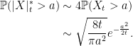 |
(1) |
The last expression here is just using the fact that Xt is centered Gaussian with variance t and applying a standard approximation for the cumulative normal distribution function.
For small values of a, approximation (1) does not work well at all. We know that the left-hand-side should tend to 1, whereas 4ℙ(Xt > a) will tend to 2, and the final expression diverges. In fact, it can be shown that
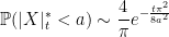 |
(2) |
as a → 0. I gave a direct proof in this math.stackexchange answer. In this post, I will look at how we can compute joint distributions of the minimum, maximum and terminal value of Brownian motion, from which limits such as (2) will follow. Continue reading “The Minimum and Maximum of Brownian motion”


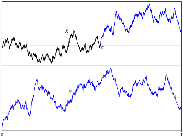
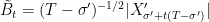


![{[0,T]}](https://s0.wp.com/latex.php?latex=%7B%5B0%2CT%5D%7D&bg=ffffff&fg=000000&s=0&c=20201002) is continuous and equal to zero at both endpoints, we can consider extending to the entire real line by partitioning the real numbers into intervals of length T and replicating the path of the process across each of these. This will result in continuous and periodic sample paths, suggesting another method of representing Brownian bridges. That is, by Fourier expansion. As we will see, the Fourier coefficients turn out to be independent normal random variables, giving a useful alternative method of constructing a Brownian bridge.
is continuous and equal to zero at both endpoints, we can consider extending to the entire real line by partitioning the real numbers into intervals of length T and replicating the path of the process across each of these. This will result in continuous and periodic sample paths, suggesting another method of representing Brownian bridges. That is, by Fourier expansion. As we will see, the Fourier coefficients turn out to be independent normal random variables, giving a useful alternative method of constructing a Brownian bridge.![{[0,1]}](https://s0.wp.com/latex.php?latex=%7B%5B0%2C1%5D%7D&bg=ffffff&fg=000000&s=0&c=20201002) . This does not reduce the generality, since bridges on an interval
. This does not reduce the generality, since bridges on an interval 
 , where
  is an IID sequence of standard normals. This series converges uniformly in t, both with probability one and in the
  norm for all
  .
. 
 be a fixed time. Then, the process
 is independent from
  .
.  , we just need to show that
 ![{{\mathbb E}[B_sX_t]}](https://s0.wp.com/latex.php?latex=%7B%7B%5Cmathbb+E%7D%5BB_sX_t%5D%7D&bg=ffffff&fg=000000&s=0&c=20201002) is zero. Using the covariance structure
is zero. Using the covariance structure ![{{\mathbb E}[X_sX_t]=s\wedge t}](https://s0.wp.com/latex.php?latex=%7B%7B%5Cmathbb+E%7D%5BX_sX_t%5D%3Ds%5Cwedge+t%7D&bg=ffffff&fg=000000&s=0&c=20201002) we obtain,
we obtain,![\displaystyle {\mathbb E}[B_sX_t]={\mathbb E}[X_sX_t]-\frac sT{\mathbb E}[X_TX_t]=s-\frac sTT=0](https://s0.wp.com/latex.php?latex=%5Cdisplaystyle++%7B%5Cmathbb+E%7D%5BB_sX_t%5D%3D%7B%5Cmathbb+E%7D%5BX_sX_t%5D-%5Cfrac+sT%7B%5Cmathbb+E%7D%5BX_TX_t%5D%3Ds-%5Cfrac+sTT%3D0+&bg=ffffff&fg=000000&s=0&c=20201002)
![{\{B_t\}_{t\in[0,T]}}](https://s0.wp.com/latex.php?latex=%7B%5C%7BB_t%5C%7D_%7Bt%5Cin%5B0%2CT%5D%7D%7D&bg=ffffff&fg=000000&s=0&c=20201002) is a Brownian bridge on the interval
is a Brownian bridge on the interval  for a standard Brownian motion X.
 , then B is called a standard Brownian bridge.
  . See lemma
  and
and  , and that their covariance is c. Then, the characteristic function of
![\displaystyle \begin{aligned} {\mathbb E}\left[e^{iaX+ibY}\right] &=e^{ia\mu_X+ib\mu_Y-\frac12(a^2\sigma_X^2+2abc+b^2\sigma_Y^2)}\\ &=e^{-abc}{\mathbb E}\left[e^{iaX}\right]{\mathbb E}\left[e^{ibY}\right] \end{aligned}](https://s0.wp.com/latex.php?latex=%5Cdisplaystyle++%5Cbegin%7Baligned%7D+%7B%5Cmathbb+E%7D%5Cleft%5Be%5E%7BiaX%2BibY%7D%5Cright%5D+%26%3De%5E%7Bia%5Cmu_X%2Bib%5Cmu_Y-%5Cfrac12%28a%5E2%5Csigma_X%5E2%2B2abc%2Bb%5E2%5Csigma_Y%5E2%29%7D%5C%5C+%26%3De%5E%7B-abc%7D%7B%5Cmathbb+E%7D%5Cleft%5Be%5E%7BiaX%7D%5Cright%5D%7B%5Cmathbb+E%7D%5Cleft%5Be%5E%7BibY%7D%5Cright%5D+%5Cend%7Baligned%7D+&bg=ffffff&fg=000000&s=0&c=20201002)
 . It is standard that the joint characteristic function of a pair of random variables is equal to the product of their characteristic functions if and only if they are independent which, in this case, corresponds to the covariance c being zero. ⬜
 is not normal.
 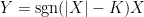 for some fixed
  , which is standard normal whenever X is. As explained in the previous post, the intermediate value theorem ensures that there is a unique value for K making the covariance
 ![{{\mathbb E}[XY]}](https://s0.wp.com/latex.php?latex=%7B%7B%5Cmathbb+E%7D%5BXY%5D%7D&bg=ffffff&fg=000000&s=0&c=20201002) equal to zero.
equal to zero.  to be jointly normal? We could simply require each of them to be normal, but this says very little about their joint distribution and is not much help in handling expressions involving more than one of the
  at once. In case that the random variables are independent, the following result is a very useful property of the normal distribution. All random variables in this post will be real-valued, except where stated otherwise, and we assume that they are defined with respect to some underlying probability space
  .
. is a sequence of independent normal random variables and
  are real numbers, then
  is normal. Let us suppose that
  has mean
  and variance
  . Then, the characteristic function of Y can be computed using the independence property and the
 ![\displaystyle \begin{aligned} {\mathbb E}\left[e^{i\lambda Y}\right] &={\mathbb E}\left[\prod_ke^{i\lambda a_k X_k}\right] =\prod_k{\mathbb E}\left[e^{i\lambda a_k X_k}\right]\\ &=\prod_ke^{-\frac12\lambda^2a_k^2\sigma_k^2+i\lambda a_k\mu_k} =e^{-\frac12\lambda^2\sigma^2+i\lambda\mu} \end{aligned}](https://s0.wp.com/latex.php?latex=%5Cdisplaystyle++%5Cbegin%7Baligned%7D+%7B%5Cmathbb+E%7D%5Cleft%5Be%5E%7Bi%5Clambda+Y%7D%5Cright%5D+%26%3D%7B%5Cmathbb+E%7D%5Cleft%5B%5Cprod_ke%5E%7Bi%5Clambda+a_k+X_k%7D%5Cright%5D+%3D%5Cprod_k%7B%5Cmathbb+E%7D%5Cleft%5Be%5E%7Bi%5Clambda+a_k+X_k%7D%5Cright%5D%5C%5C+%26%3D%5Cprod_ke%5E%7B-%5Cfrac12%5Clambda%5E2a_k%5E2%5Csigma_k%5E2%2Bi%5Clambda+a_k%5Cmu_k%7D+%3De%5E%7B-%5Cfrac12%5Clambda%5E2%5Csigma%5E2%2Bi%5Clambda%5Cmu%7D+%5Cend%7Baligned%7D+&bg=ffffff&fg=000000&s=0&c=20201002)
 and
and  . This is the characteristic function of a normal random variable with mean
  and variance
  . ⬜
. ⬜ of real-valued random variables is multivariate normal (or joint normal) if and only if all of its finite linear combinations are normal.

 . By the theory of
  multiplied by a function of x over the range
  . In fact, this can be done in a way such that the function of x is a probability density function, and hence expresses the Riemann zeta function over the entire complex plane in terms of the generating function
 ![{{\mathbb E}[X^s]}](https://s0.wp.com/latex.php?latex=%7B%7B%5Cmathbb+E%7D%5BX%5Es%5D%7D&bg=ffffff&fg=000000&s=0&c=20201002) of a positive random variable X. The probability distributions involved here are not the standard ones taught to students of probability theory, so may be new to many people. Although these distributions are intimately related to the Riemann zeta function they also, intriguingly, turn up in seemingly unrelated contexts involving Brownian motion.
of a positive random variable X. The probability distributions involved here are not the standard ones taught to students of probability theory, so may be new to many people. Although these distributions are intimately related to the Riemann zeta function they also, intriguingly, turn up in seemingly unrelated contexts involving Brownian motion.
 is the correct value for this to be true, it is the one fact that I state here without proof.
  and
and  have the same distribution, so that they have the same mean and, therefore,
 ![{{\mathbb E}[X]=0}](https://s0.wp.com/latex.php?latex=%7B%7B%5Cmathbb+E%7D%5BX%5D%3D0%7D&bg=ffffff&fg=000000&s=0&c=20201002) .
.
![\displaystyle \begin{aligned} {\mathbb E}[X^2] &=\int x^2\varphi(x)dx\\ &= -\int x\varphi^\prime(x)dx\\ &=\int\varphi(x)dx-[x\varphi(x)]_{-\infty}^\infty=1 \end{aligned}](https://s0.wp.com/latex.php?latex=%5Cdisplaystyle++%5Cbegin%7Baligned%7D+%7B%5Cmathbb+E%7D%5BX%5E2%5D+%26%3D%5Cint+x%5E2%5Cvarphi%28x%29dx%5C%5C+%26%3D+-%5Cint+x%5Cvarphi%5E%5Cprime%28x%29dx%5C%5C+%26%3D%5Cint%5Cvarphi%28x%29dx-%5Bx%5Cvarphi%28x%29%5D_%7B-%5Cinfty%7D%5E%5Cinfty%3D1+%5Cend%7Baligned%7D+&bg=ffffff&fg=000000&s=0&c=20201002)

 be measurable. Then, for all
  ,
, ![\displaystyle \begin{aligned} {\mathbb E}[e^{\lambda X}f(X)] &={\mathbb E}[e^{\lambda X}]{\mathbb E}[f(X+\lambda)]\\ &=e^{\frac{\lambda^2}{2}}{\mathbb E}[f(X+\lambda)]. \end{aligned}](https://s0.wp.com/latex.php?latex=%5Cdisplaystyle++%5Cbegin%7Baligned%7D+%7B%5Cmathbb+E%7D%5Be%5E%7B%5Clambda+X%7Df%28X%29%5D+%26%3D%7B%5Cmathbb+E%7D%5Be%5E%7B%5Clambda+X%7D%5D%7B%5Cmathbb+E%7D%5Bf%28X%2B%5Clambda%29%5D%5C%5C+%26%3De%5E%7B%5Cfrac%7B%5Clambda%5E2%7D%7B2%7D%7D%7B%5Cmathbb+E%7D%5Bf%28X%2B%5Clambda%29%5D.+%5Cend%7Baligned%7D+&bg=ffffff&fg=000000&s=0&c=20201002)
