In filtering theory, we have a filtered probability space  and a signal process
  . The sigma-algebra
  represents the collection of events which are observable up to and including time t. The process X is not assumed to be adapted, so need not be directly observable. For example, we may only be able to measure an observation process
  , which incorporates some noise
  , and generates the filtration , so is adapted. The problem, then, is to compute an estimate for
  based on the observable data at time t. Looking at the expected value of X conditional on the observable data, we obtain the following estimate for X at each time
  ,
,
![\displaystyle Y_t={\mathbb E}[X_t\;\vert\mathcal{F}_t]{\rm\ \ (a.s.)}](https://s0.wp.com/latex.php?latex=%5Cdisplaystyle++Y_t%3D%7B%5Cmathbb+E%7D%5BX_t%5C%3B%5Cvert%5Cmathcal%7BF%7D_t%5D%7B%5Crm%5C+%5C+%28a.s.%29%7D+&bg=ffffff&fg=000000&s=0&c=20201002) |
(1) |
The process Y is adapted. However, as (1) only defines Y up to a zero probability set, it does not give us the paths of Y, which requires specifying its values simultaneously at the uncountable set of times in  . Consequently, (1) does not tell us the distribution of Y at random times. So, it is necessary to specify a good version for Y.
Optional projection gives a uniquely defined process which satisfies (1), not just at every time t in , but also at all stopping times. The full theory of optional projection for jointly measurable processes requires the optional section theorem. As I will demonstrate, in the case where X is right-continuous, optional projection can be done by more elementary methods.
Throughout this post, it will be assumed that the underlying filtered probability space satisfies the usual conditions, meaning that it is complete and right-continuous,  . Stochastic processes are considered to be defined up to evanescence. That is, two processes are considered to be the same if they are equal up to evanescence. In order to apply (1), some integrability requirements need to imposed on X. Often, to avoid such issues, optional projection is defined for uniformly bounded processes. For a bit more generality, I will relax this requirement a bit and use prelocal integrability. Recall that, in these notes, a process X is prelocally integrable if there exists a sequence of stopping times
  increasing to infinity and such that
 |
(2) |
is integrable. This is a strong enough condition for the conditional expectation (1) to exist, not just at each fixed time, but also whenever t is a stopping time. The main result of this post can now be stated.
Theorem 1 (Optional Projection) Let X be a right-continuous and prelocally integrable process. Then, there exists a unique right-continuous process Y satisfying (1).
Uniqueness is immediate, as (1) determines Y, almost-surely, at each fixed time, and this is enough to uniquely determine right-continuous processes up to evanescence. Existence of Y is the important part of the statement, and the proof will be left until further down in this post.
The process defined by Theorem 1 is called the optional projection of X, and is denoted by  . That is, is the unique right-continuous process satisfying
![\displaystyle {}^{\rm o}\!X_t={\mathbb E}[X_t\;\vert\mathcal{F}_t]{\rm\ \ (a.s.)}](https://s0.wp.com/latex.php?latex=%5Cdisplaystyle++%7B%7D%5E%7B%5Crm+o%7D%5C%21X_t%3D%7B%5Cmathbb+E%7D%5BX_t%5C%3B%5Cvert%5Cmathcal%7BF%7D_t%5D%7B%5Crm%5C+%5C+%28a.s.%29%7D+&bg=ffffff&fg=000000&s=0&c=20201002) |
(3) |
for all times t. In practise, the process X will usually not just be right-continuous, but will also have left limits everywhere. That is, it is cadlag.
Theorem 2 Let X be a cadlag and prelocally integrable process. Then, its optional projection is cadlag.
A simple example of optional projection is where is constant in t and equal to an integrable random variable U. Then,  is the cadlag version of the martingale
 ![{{\mathbb E}[U\;\vert\mathcal{F}_t]}](https://s0.wp.com/latex.php?latex=%7B%7B%5Cmathbb+E%7D%5BU%5C%3B%5Cvert%5Cmathcal%7BF%7D_t%5D%7D&bg=ffffff&fg=000000&s=0&c=20201002) . Continue reading “Optional Projection For Right-Continuous Processes” →
. Continue reading “Optional Projection For Right-Continuous Processes” →
 .
.

 such that
  is convex in x and right-continuous and decreasing in t, is
  necessarily a semimartingale? It was explained how this is equivalent to the
 ![{f\colon[0,1]^2\rightarrow{\mathbb R}}](https://s0.wp.com/latex.php?latex=%7Bf%5Ccolon%5B0%2C1%5D%5E2%5Crightarrow%7B%5Cmathbb+R%7D%7D&bg=ffffff&fg=000000&s=0&c=20201002) such that
such that  where
where  and
and  are convex in x and increasing in t. This is the form of the hypothesis which this post will be concerned with, so the example will only involve simple real analysis and no stochastic calculus. I will give some numerical calculations suggesting that the construction below is a counterexample, but do not have any proof of this. So, the hypothesis is still open.
![{\{M_t\}_{t\in[0,1]}}](https://s0.wp.com/latex.php?latex=%7B%5C%7BM_t%5C%7D_%7Bt%5Cin%5B0%2C1%5D%7D%7D&bg=ffffff&fg=000000&s=0&c=20201002) is the martingale constructed there, then
is the martingale constructed there, then![\displaystyle C(t,x)={\mathbb E}[(M_t-x)_+]](https://s0.wp.com/latex.php?latex=%5Cdisplaystyle++C%28t%2Cx%29%3D%7B%5Cmathbb+E%7D%5B%28M_t-x%29_%2B%5D+&bg=ffffff&fg=000000&s=0&c=20201002)
![{[0,1]\times[-1,1]}](https://s0.wp.com/latex.php?latex=%7B%5B0%2C1%5D%5Ctimes%5B-1%2C1%5D%7D&bg=ffffff&fg=000000&s=0&c=20201002) to
to  which is convex in x and increasing in t. The question is then whether C can be expressed as the difference of functions which are convex in x and decreasing in t. The example constructed in this post will be the same as C with the time direction reversed, and with a linear function of x added so that it is zero at
  .
. 
 . That is,
  at all times outside of the set of nontrivial intervals on which M is constant. Expressed in terms of the
  on the set
  and,
and,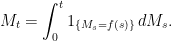
 where M is a martingale as above. From this, we can infer that

 . In the case where f is twice continuously differentiable then the process V is given by
  is a uniformly bounded
 -integrable martingale, any
  , then
  is enough to guarantee that Y is a martingale. Also, it is a
  to denote the running absolute maximum of a cadlag martingale X, then
  is
is  is. It is natural to ask whether this also holds for
  . As martingales are integrable by definition, this is just asking whether cadlag martingales necessarily have an integrable maximum. Integrability of the maximum process does have some important consequences in the theory of martingales. By the
 ![{[X]^{1/2}}](https://s0.wp.com/latex.php?latex=%7B%5BX%5D%5E%7B1%2F2%7D%7D&bg=ffffff&fg=000000&s=0&c=20201002) , being integrable. Stochastic integration over bounded integrands
, being integrable. Stochastic integration over bounded integrands 
 . Here,
  denotes the standard
 ![{\lVert U\rVert_p\equiv{\mathbb E}[U^p]^{1/p}}](https://s0.wp.com/latex.php?latex=%7B%5ClVert+U%5CrVert_p%5Cequiv%7B%5Cmathbb+E%7D%5BU%5Ep%5D%5E%7B1%2Fp%7D%7D&bg=ffffff&fg=000000&s=0&c=20201002) .
. in (
in ( there exists a strictly positive cadlag
 ![{\{X_t\}_{t\in[0,1]}}](https://s0.wp.com/latex.php?latex=%7B%5C%7BX_t%5C%7D_%7Bt%5Cin%5B0%2C1%5D%7D%7D&bg=ffffff&fg=000000&s=0&c=20201002) with
with  .
.  . So, supposing that (
 in place of
  . By choosing
  as close to
  and
and 
 and
and  ,
, ![\displaystyle {\mathbb P}\left(X^*_t\ge x\right)\le\inf_{y < x}\frac{{\mathbb E}\left[(X_t-y)_+\right]}{x-y}.](https://s0.wp.com/latex.php?latex=%5Cdisplaystyle++%7B%5Cmathbb+P%7D%5Cleft%28X%5E%2A_t%5Cge+x%5Cright%29%5Cle%5Cinf_%7By+%3C+x%7D%5Cfrac%7B%7B%5Cmathbb+E%7D%5Cleft%5B%28X_t-y%29_%2B%5Cright%5D%7D%7Bx-y%7D.+&bg=ffffff&fg=000000&s=0&c=20201002)
 , and then it immediately follows for the infimum. Choosing
  , consider the
 and
and  whenever
  . As
. As  is nonnegative and increasing in z, this means that
  is bounded above by
  . Taking expectations,
![\displaystyle {\mathbb P}\left(X^*_t\ge x\right)\le{\mathbb E}\left[f(X_{\tau\wedge t})\right]/f(x^\prime).](https://s0.wp.com/latex.php?latex=%5Cdisplaystyle++%7B%5Cmathbb+P%7D%5Cleft%28X%5E%2A_t%5Cge+x%5Cright%29%5Cle%7B%5Cmathbb+E%7D%5Cleft%5Bf%28X_%7B%5Ctau%5Cwedge+t%7D%29%5Cright%5D%2Ff%28x%5E%5Cprime%29.+&bg=ffffff&fg=000000&s=0&c=20201002)

![\displaystyle {\mathbb P}\left(X^*_t\ge x\right)\le{\mathbb E}\left[f(X_t)\right]/f(x^\prime).](https://s0.wp.com/latex.php?latex=%5Cdisplaystyle++%7B%5Cmathbb+P%7D%5Cleft%28X%5E%2A_t%5Cge+x%5Cright%29%5Cle%7B%5Cmathbb+E%7D%5Cleft%5Bf%28X_t%29%5Cright%5D%2Ff%28x%5E%5Cprime%29.+&bg=ffffff&fg=000000&s=0&c=20201002)
 increase to
  gives the result. ⬜
 is a probability measure on
  and
and  then there exists a continuous martingale X (defined on some
 ![\displaystyle \setlength\arraycolsep{2pt} \begin{array}{rl} \displaystyle [X]_t&\displaystyle=[X]^c_t+\sum_{s\le t}(\Delta X_s)^2,\smallskip\\ \displaystyle [X,Y]_t&\displaystyle=[X,Y]^c_t+\sum_{s\le t}\Delta X_s\Delta Y_s. \end{array}](https://s0.wp.com/latex.php?latex=%5Cdisplaystyle++%5Csetlength%5Carraycolsep%7B2pt%7D+%5Cbegin%7Barray%7D%7Brl%7D+%5Cdisplaystyle+%5BX%5D_t%26%5Cdisplaystyle%3D%5BX%5D%5Ec_t%2B%5Csum_%7Bs%5Cle+t%7D%28%5CDelta+X_s%29%5E2%2C%5Csmallskip%5C%5C+%5Cdisplaystyle+%5BX%2CY%5D_t%26%5Cdisplaystyle%3D%5BX%2CY%5D%5Ec_t%2B%5Csum_%7Bs%5Cle+t%7D%5CDelta+X_s%5CDelta+Y_s.+%5Cend%7Barray%7D+&bg=ffffff&fg=000000&s=0&c=20201002)
![{[X]^c}](https://s0.wp.com/latex.php?latex=%7B%5BX%5D%5Ec%7D&bg=ffffff&fg=000000&s=0&c=20201002) , is zero. As the only difference between the
, is zero. As the only difference between the ![{[X]^c=0}](https://s0.wp.com/latex.php?latex=%7B%5BX%5D%5Ec%3D0%7D&bg=ffffff&fg=000000&s=0&c=20201002) .
. ![{[X,Y]^c=0}](https://s0.wp.com/latex.php?latex=%7B%5BX%2CY%5D%5Ec%3D0%7D&bg=ffffff&fg=000000&s=0&c=20201002) for all semimartingales Y.
for all semimartingales Y. ![{[X,Y]=0}](https://s0.wp.com/latex.php?latex=%7B%5BX%2CY%5D%3D0%7D&bg=ffffff&fg=000000&s=0&c=20201002) for all continuous semimartingales Y.
for all continuous semimartingales Y. ![{[X,M]=0}](https://s0.wp.com/latex.php?latex=%7B%5BX%2CM%5D%3D0%7D&bg=ffffff&fg=000000&s=0&c=20201002) for all continuous local martingales M.
for all continuous local martingales M.  for a
for a  of FV processes such that
  in the