Properties of Quadratic Variations

George Lowther Stochastic Calculus Notes, Stochastic Integration 19 January 1016 September 20

Being able to handle quadratic variations and covariations of processes is very important in stochastic calculus. Apart from appearing in the integration by parts formula, they are required for the stochastic change of variables formula, known as Ito’s lemma, which will be the subject of the next post. Quadratic covariations satisfy several simple relations which make them easy to handle, especially in conjunction with the stochastic integral.

Recall from the previous post that the covariation ${[X,Y]}$ is a cadlag adapted process, so that its jumps ${\Delta [X,Y]_t\equiv [X,Y]_t-[X,Y]_{t-}}$ are well defined.

Lemma 1 If ${X,Y}$ are semimartingales then

$\displaystyle \Delta [X,Y]=\Delta X\Delta Y.$ (1)

In particular, ${\Delta [X]=\Delta X^2}$ .

Proof: Taking the jumps of the integration by parts formula for ${XY}$ gives

$\displaystyle \Delta XY = X_{-}\Delta Y + Y_{-}\Delta X + \Delta [X,Y],$

and rearranging this gives the result. ⬜

An immediate consequence is that quadratic variations and covariations involving continuous processes are continuous. Another consequence is that the sum of the squares of the jumps of a semimartingale over any bounded interval must be finite.

Corollary 2 Every semimartingale ${X}$ satisfies

$\displaystyle \sum_{s\le t}\Delta X^2_s\le [X]_t<\infty.$

Proof: As ${[X]}$ is increasing, the inequality ${[X]_t\ge \sum_{s\le t}\Delta [X]_s}$ holds. Substituting in ${\Delta[X]=\Delta X^2}$ gives the result. ⬜

Next, the following result shows that covariations involving continuous finite variation processes are zero. As Lebesgue-Stieltjes integration is only defined for finite variation processes, this shows why quadratic variations do not play an important role in standard calculus. For noncontinuous finite variation processes, the covariation must have jumps satisfying (1), so will generally be nonzero. In this case, the covariation is just given by the sum over these jumps. Integration with respect to any FV process ${V}$ can be defined as the Lebesgue-Stieltjes integral on the sample paths, which is well defined for locally bounded measurable integrands and, when the integrand is predictable, agrees with the stochastic integral.

Lemma 3 Let ${X}$ be a semimartingale and ${V}$ be an FV process. Their covariation is

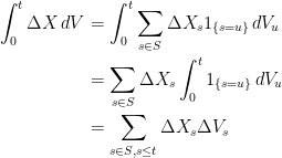
$\displaystyle [X,V]_t = \int_0^t \Delta X\,dV = \sum_{s\le t}\Delta X_s\Delta V_s.$ (2)

In particular, if either of ${X}$ or ${V}$ is continuous then ${[X,V]=0}$ .

Proof: Expressing the covariation as the limit along equally spaced partitions of ${[0,t]}$ gives

$\displaystyle \setlength\arraycolsep{2pt} \begin{array}{rl} \displaystyle [X,V]_t &\displaystyle= \lim_{n\rightarrow\infty}\sum_{k=1}^n (X_{kt/n}-X_{(k-1)t/n})(V_{kt/n}-V_{(k-1)t/n})\smallskip\\ &\displaystyle=\lim_{n\rightarrow\infty}\sum_{k=1}^n\int_0^t 1_{\{(k-1)t/n<s\le kt/n\}}(X_{kt/n}-X_{(k-1)t/n})\,dV_s\smallskip\\ &\displaystyle=\int_0^t\lim_{n\rightarrow\infty}\sum_{k=1}^n 1_{\{(k-1)t/n<s\le kt/n\}}(X_{kt/n}-X_{(k-1)t/n})\,dV_s\smallskip\\ &\displaystyle=\int_0^t\Delta X_s\,dV_s. \end{array}$

The third equality here makes use of the bounded convergence theorem to commute the limit with the integral sign. Then, as ${X}$ is cadlag, on each sample path there is only a countable set of times ${S}$ at which ${\Delta X\not=0}$ . Bounded convergence can again be used to evaluate the integral,

$\displaystyle \setlength\arraycolsep{2pt} \begin{array}{rl} \displaystyle\int_0^t\Delta X\,dV &\displaystyle= \int_0^t \sum_{s\in S}\Delta X_s1_{\{s=u\}}\,dV_u\smallskip\\ &\displaystyle=\sum_{s\in S}\Delta X_s\int_0^t 1_{\{s=u\}}\,dV_u\smallskip\\ &\displaystyle=\sum_{s\in S, s\le t} \Delta X_s\Delta V_s \end{array}$

as required. ⬜

If ${X,Y}$ are semimartingales and ${V,W}$ are continuous FV processes then,

$\displaystyle [X+V,Y+W]=[X,Y].$

That is, when calculating covariations, we can disregard any continuous FV terms added to the processes. A consequence of Lemma 3 is that the standard integration by parts formula, with no covariation term, applies whenever either of the two processes has finite variation. The integral with respect to the FV process ${V}$ in the following is the Lebesgue-Stieltjes integral on the sample paths. As ${X}$ need not be predictable, it is not always defined as a stochastic integral.

Corollary 4 Let ${X}$ be a semimartingale and ${V}$ be an FV process. Then,

$\displaystyle XV = X_0V_0+\int X\,dV + \int V_-\,dX.$

Proof: Substitute (2) for the covariation term in the integration by parts formula to get the following

$\displaystyle XV = X_0V_0 +\int V_-\,dX + \int X_-\,dV + \int \Delta X\,dV.$

The final two integrals on the right hand side can be combined into a single integral of ${X_-+\Delta X=X}$ , giving the result. ⬜

A d-dimensional process ${X=(X^1,\ldots,X^d)}$ is said to be a semimartingale if each of its components ${X^i}$ are semimartingales. The quadratic variation ${[X]}$ is defined as the dxd matrix-valued process

$\displaystyle [X]^{ij}\equiv [X^i,X^j].$

This will also be increasing, in the sense that ${[X]_t-[X]_s}$ is almost surely positive semidefinite for all times ${t>s}$ . That is,

$\displaystyle \lambda^{\rm t}[X]\lambda = \lambda^i\lambda^j[X^i,X^j]=\left[\lambda\cdot X\right]$

is increasing for all vectors ${\lambda\in{\mathbb R}^n}$ . Here, I am using the summation convention, where the indices appearing twice in a single term are summed over. This gives the following result for the integral with respect to ${[X]}$ .

Lemma 5 Let ${X^1,\ldots,X^d}$ be semimartingales and ${\xi^1,\ldots,\xi^d}$ be bounded and measurable processes. Then,

$\displaystyle \int \xi^i\xi^j\,d[X^i,X^j]$ (3)

is an increasing process.

Proof: Almost surely, ${[X]}$ is an increasing matrix valued process, as mentioned above. Restricting to any fixed sample path satisfying this property, consider a process of the form

$\displaystyle \xi_t = c_01_{\{t=0\}} +\sum_{k=1}^n c_k 1_{\{t_{k-1}<t\le t_k\}}$

(4)

for ${c_0,\ldots,c_n\in{\mathbb R}^d}$ and times ${0=t_0\le\cdots\le t_n}$ . This has integral

$\displaystyle \setlength\arraycolsep{2pt} \begin{array}{rl} \displaystyle\int_0^t \xi^i\xi^j\,d[X^i,X^j] &\displaystyle= \sum_{k=1}^n \int_0^t 1_{\{t_{k-1}<s\le t_{k-1}\}}c^i_kc^j_k\,d[X^i,X^j]_s\smallskip\\ &\displaystyle=\sum_{k=1}^n c^{\rm t}_k([X]_{t\wedge t_k}-[X]_{t\wedge t_{k-1}})c_k \end{array}$

which is increasing. The idea is to apply the functional monotone class theorem to extend this to all bounded and measurable processes. So, let ${V}$ be the set of bounded measurable functions for which (3) gives an increasing process. By the argument above, this includes all step functions of the form (4). By the monotone class theorem, to show that ${V}$ contains all bounded measurable functions it is enough to show that if ${\xi^n\in V}$ is a uniformly bounded sequence tending to the limit ${\xi}$ , then ${\xi\in V}$ . However, this follows from the bounded convergence theorem for the Lebesgue-Stieltjes integrals with respect to ${[X]}$ and the fact that a limit of increasing functions is increasing. ⬜

The quadratic covariation considered as a bilinear map ${(X,Y)\mapsto [X,Y]_t}$ is symmetric and positive semidefinite. The Cauchy-Schwarz inequality gives the following bound for the covariation,

$\displaystyle \vert [X,Y]\vert \le\sqrt{[X][Y]}$

More generally, the previous result can be used to obtain the Kunita-Watanabe inequality.

Theorem 6 (Kunita-Watanabe Inequality) Let ${X,Y}$ be semimartingales and ${\alpha,\beta}$ be measurable processes. Then,

$\displaystyle \int_0^t\vert\alpha\beta\vert\,\vert d[X,Y]\vert\le\sqrt{\int_0^t\alpha^2\,d[X]\,\int_0^t\beta^2\,d[Y]}.$

Proof: First, suppose that ${\alpha,\beta}$ are bounded. Considering the 2-dimensional semimartingale ${Z=(X,Y)}$ and ${\xi=(\lambda\alpha,\pm\beta)}$ for a fixed ${\lambda>0}$ , the previous result says that

$\displaystyle \lambda^2\int\alpha^2\,d[X]+\int\beta^2\,d[Y]\pm 2\lambda\int\alpha\beta\,d[X,Y]$

is an increasing process. As the first two terms are increasing, and the variation of the third term is ${2\lambda\int\vert\alpha\beta\vert\,\vert d[X,Y]\vert}$ this gives the following inequality,

$\displaystyle 2\lambda\int_0^t\vert\alpha\beta\vert\,\vert d[X,Y]\vert\le \lambda^2\int_0^t\alpha^2\,d[X]+\int_0^t\beta^2\,d[Y].$

The result follows by setting ${\lambda=(\int_0^t\alpha^2\,d[X])^{-1/2}(\int_0^t\beta^2\,d[Y])^{1/2}}$ . Finally, this extends to unbounded integrands by monotone convergence. ⬜

For example, consider standard Brownian motions ${B^1,B^2}$ . These have quadratic variation ${[B^1]_t=[B^2]_t=t}$ and the Kunita-Watanabe inequality says that

$\displaystyle \int\xi^2\,\vert d[B^1,B^2]\vert \le \int\xi^2\,dt.$

The Radon-Nikodym theorem can then be used to imply the existence of a predictable process ${\vert\rho_t\vert\le 1}$ with ${d[B^1,B^2]=\rho\,dt}$ . This is the instantaneous correlation of the Brownian motions. Recall from the previous post that this is consistent with the quadratic covariations where the correlation is a fixed number.

We now arrive at the following result allowing us to commute the order in which stochastic integrals and quadratic covariations are calculated. This is a very useful result which is often required when manipulating stochastic integrals. Note that equations (6) and (7) can be written in differential form as follows,

$\displaystyle \setlength\arraycolsep{2pt} \begin{array}{rl} \displaystyle (\xi\,dX)dY &\displaystyle= \xi\,(dXdY),\smallskip\\ \displaystyle (\xi\,dX)^2 &\displaystyle= \xi^2\,dX^2. \end{array}$

Theorem 7 Let ${X,Y}$ be semimartingales and ${\xi}$ be an ${X}$ -integrable process. Then, ${\xi}$ is ${[X,Y]}$ -integrable in the Lebesgue-Stieltjes sense,

$\displaystyle \int_0^t\vert\xi\vert\,\vert d[X,Y]\vert<\infty$ (5)

and,

$\displaystyle \left[\int\xi\,dX,Y\right] = \int\xi\,d[X,Y].$ (6)

Furthermore, the quadratic variation of ${\int\xi\,dX}$ is given by,

$\displaystyle \left[\int\xi\,dX\right]=\int\xi^2\,d[X].$ (7)

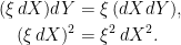
As an example, consider Ito processes ${X,Y}$ ,

$\displaystyle dX_t = \alpha\,dB^1_t+\mu\,dt,\ dY_t = \beta\,dB^2_t+\nu\,dt$

where ${B^1,B^2}$ are Brownian motions with correlation ${\rho}$ , so ${dB^1dB^2=\rho dt}$ . As mentioned above, the continuous finite variation parts ${\mu\,dt}$ and ${\nu\,dt}$ do not contribute to the covariation. Theorem 7 gives,

$\displaystyle d[X,Y] = (\alpha\,dB^1)(\beta\,dB^2)=\alpha\beta\,dB^1dB^2 = \alpha\beta\rho\,dt.$

The proof of Theorem 7 is as follows.

Proof: First, consider the case where ${\xi}$ is an elementary predictable process, so that it is left-continuous and piecewise constant, with discontinuities at some finite set of times ${S}$ . Setting ${Z\equiv\int\xi\,dX}$ then ${Z_t-Z_s=\xi_t(X_t-X_s)}$ for any interval ${(s,t]}$ over which ${\xi}$ is constant. Then, the covariation calculated along a partition ${P=\{0=\tau_0\le\tau_1\le\cdots\uparrow\infty\}}$ containing ${S}$ satisfies,

$\displaystyle \setlength\arraycolsep{2pt} \begin{array}{rl} \displaystyle [Z,Y]^P_t &\displaystyle= \sum_{n=1}^\infty (Z_{\tau_n\wedge t}-Z_{\tau_{n-1}\wedge t})(Y_{\tau_n\wedge t}-Y_{\tau_{n-1}\wedge t})\smallskip\\ &\displaystyle=\sum_{n=1}^\infty \xi_{\tau_n}(X_{\tau_n\wedge t}-X_{\tau_{n-1}\wedge t})(Y_{\tau_n\wedge t}-Y_{\tau_{n-1}\wedge t})\smallskip\\ &\displaystyle=\int_0^t\xi\,d[X,Y]^P. \end{array}$

Taking the limit of such partitions gives (6).

Now, let ${V}$ be the set of processes ${\xi\in L^1(X)\cap L^1([X,Y])}$ such that (6) is satisfied. As just shown, this includes the elementary predictable processes. The idea is to apply the functional monotone class theorem to prove that ${V=L^1(X)}$ .

Let ${\xi^n\in V}$ be a sequence converging to a limit ${\xi\in L^1([X,Y])}$ , and dominated by some ${\alpha\in L^1(X)}$ . Setting ${Z^n=\int\xi^n\,dX}$ , integration by parts gives

$\displaystyle \int\xi^n\,d[X,Y]=[Z^n,Y] =Z^nY - \int_0^tY_-\xi^n\,dX-\int Z^n_-\,dY.$

(8)

By the dominated convergence theorem, the first two terms on the right converge ucp to the limit with ${\xi}$ and ${Z\equiv\int\xi\,dX}$ in place of ${\xi^n}$ and ${Z^n}$ . Furthermore, as ${Z^n\xrightarrow{ucp}Z}$ , we may pass to a subsequence such that this almost surely converges uniformly on compacts. Then, the dominated convergence theorem shows that the final term on the right hand side of (8) also converges to the limit with ${Z}$ in place of ${Z^n}$ . Taking the limit ${n\rightarrow\infty}$ and applying integration by parts a second time gives,

$\displaystyle \int\xi^n\,d[X,Y] \xrightarrow{ucp} ZY-\int_0^t Y_-\xi\,dX-\int Z_-\,dY = \left[\int\xi\,dX,Y\right].$

(9)

In particular, if ${\xi^n}$ is a uniformly bounded sequence then applying bounded convergence to the left hand side gives (6), so that ${\xi\in V}$ . The monotone class theorem then says that ${V}$ contains all bounded predictable processes.

Next, suppose that ${\xi^n\rightarrow 0}$ are bounded predictable processes dominated by ${\alpha\in L^1(X)}$ . Then, (9) says that ${\int\xi^n\,d[X,Y]\rightarrow 0}$ and, by definition, ${\alpha}$ is ${[X,Y]}$ -integrable in the sense of stochastic integration. Therefore, ${L^1(X)\subseteq L^1([X,Y])}$ .

Any ${X}$ -integrable process ${\xi}$ is the limit of a sequence of bounded predictable processes ${\vert\xi^n\vert\le\vert\xi\vert}$ . As ${\xi\in L^1([X,Y])}$ , dominated convergence implies that left hand side of (9) tends to ${\int\xi\,d[X,Y]}$ , giving (6) as required.

So far, we have shown that every ${X}$ -integrable process ${\xi}$ is also ${[X,Y]}$ -integrable, and equation (6) is satisfied.

Setting ${Z\equiv\int\xi\,dX}$ , we have shown that ${\xi}$ is ${[X,Z]}$ -integrable and ${[Z]=\int\xi\,d[X,Z]}$ . Similarly, ${\xi}$ is ${[X]}$ -integrable satisfying ${[X,Z]=\int\xi\,d[X]}$ . So, by associativity of stochastic integration, ${\xi^2}$ is ${X}$ -integrable and equation (7) follows,

$\displaystyle \int_0^t\xi^2\,d[X]=\int_0^t\xi\,d[X,Z]=[Z]_t<\infty.$

Finally, equation (5) follows from the Kunita-Watanabe inequality,

$\displaystyle \int_0^t\vert\xi\vert\,\vert d[X,Y]\vert\le\sqrt{\int_0^t\xi^2\,d[X]_t\, [Y]_t}<\infty.$

⬜

A simple consequence of Theorem 7 is that stopping the covariation of two semimartingales at a stopping time is the same as stopping either of the individual processes.

Corollary 8 If ${X,Y}$ are semimartingales and ${\tau}$ is a stopping time then,

$\displaystyle [X,Y]^\tau = \left[X^\tau,Y\right] = \left[ X, Y^\tau\right].$

In particular, ${[X^\tau]=[X]^\tau}$ .

Proof: The result follows by integrating ${1_{(0,\tau]}}$ ,

$\displaystyle [X,Y]^\tau=\int 1_{(0,\tau]}\,d[X,Y] = \left[\int 1_{(0,\tau]}\,dX,Y\right]=[X^\tau,Y].$

⬜

A semimartingale which is small in absolute value does not necessarily have a small quadratic variation or, to state this another way, quadratic variation is not a continuous map under ucp convergence. For example, consider solutions to the stochastic differential equation ${dX=dB-\lambda X dt}$ for a Brownian motion B, constant ${\lambda > 0}$ , and initial condition ${X_0=0}$ . This is an Ornstein-Uhlenbeck process with mean reversion rate ${\lambda}$ . It can be shown that, as a function of ${\lambda}$ , the solution X will converge ucp to zero in the limit as ${\lambda\rightarrow\infty}$ , but, the quadratic variation ${[X]_t=t}$ does not depend on ${\lambda}$ at all. Continuity of quadratic variation and covariation can be recovered by, instead, using the stronger semimartingale topology. In the following, ${\mathcal{S}}$ denotes the space of semimartingales and ${X^n\xrightarrow{\rm sm}X}$ denotes convergence of a sequence ${X^n}$ to ${X}$ in the semimartingale topology.

Lemma 9 Quadratic covariation defines a jointly continuous map

$\displaystyle \setlength\arraycolsep{2pt} \begin{array}{rl} &\displaystyle \mathcal{S}\times\mathcal{S}\rightarrow\mathcal{S},\smallskip\\ &\displaystyle (X,Y)\mapsto[X,Y] \end{array}$

under the semimartingale topology.

That is, if ${\{X^n\}_{n\in{\mathbb N}}}$ , ${\{Y^n\}_{n\in{\mathbb N}}}$ , X, Y are semimartingales with ${X^n\xrightarrow{\rm sm}X}$ and ${Y^n\xrightarrow{\rm sm}Y}$ , then ${[X^n,Y^n]\xrightarrow{\rm sm}[X,Y]}$ and, furthermore, the variation of ${[X^n,Y^n]-[X,Y]}$ on any bounded interval tends to zero in probability.

Proof: We start by showing that if ${X^n\xrightarrow{\rm sm}0}$ then ${[X^n]_t\rightarrow0}$ in probability for a fixed time t. As semimartingale convergence implies ucp convergence, the stopping times

$\displaystyle \tau_n=\inf\left\{s\ge0\colon\vert X^n_s\vert\ge1\right\}$

tend to infinity in probability. So, it is enough to show that ${[X^n]_{\tau_n\wedge t}}$ tends to zero in probability. Using integration by parts,

$\displaystyle [X^n]_{\tau_n\wedge t}=(X^n_{\tau_n\wedge t})^2-(X^n_0)^2-2\int_0^t1_{(0,\tau_n]}X^n_-\,dX^n.$

The first two terms on the right hand side tend to zero in probability, by ucp convergence. For the final term, for any fixed n, note that ${1_{(0,\tau_n]}X^n_-}$ is left-continuous, adapted, and bounded by 1 and, hence, can be written as the limit of a sequence of elementary predictable processes ${\vert\xi^m\vert\le1}$ . For example, we can take ${\xi^m_s=1_{\{k/m < \tau_n\}}X^n_{k/m}}$ over ${k < ms\le k+1}$ . Recalling that ${D^{\rm sm}_t(X)}$ denotes the supremum of ${{\mathbb E}[\vert\xi_0X_0+\int_0^t\xi\,dX\vert\wedge1]}$ over bounded elementary processes ${\vert\xi\vert\le1}$ ,

$\displaystyle \setlength\arraycolsep{2pt} \begin{array}{rl} \displaystyle{\mathbb E}\left[\left\vert\int_0^t1_{(0,\tau_n]}X^n_-\,dX^n\right\vert\wedge1\right]&\displaystyle=\lim_{m\rightarrow\infty}{\mathbb E}\left[\left\vert\int_0^t\xi^m\,dX^n\right\vert\wedge1\right]\smallskip\\&\displaystyle\le D^{\rm sm}_t(X^n). \end{array}$

Here, bounded convergence has been used to write the integral as a limit of integrals over ${\xi^m}$ . By definition of the semimartingale topology, ${D^{\rm sm}_t(X^n)\rightarrow0}$ as n tends to infinity and, therefore, we have shown that ${\int_0^t1_{(0,\tau_n]}X^n_-\,dX^n}$ tends to zero in probability. So, ${[X^n]_t\rightarrow0}$ in probability as claimed.

Now suppose that ${X^n\xrightarrow{\rm sm}X}$ and ${Y^n\xrightarrow{\rm sm}Y}$ . By the bilinearity of quadratic covariations,

$\displaystyle [X^n,Y^n]-[X,Y]=[X^n-X,Y^n-Y]+[X^n-X,Y]+[X,Y^n-Y].$

Applying the Kunita-Watanabe inequality (Theorem 6) to each of the three terms on the right hand side shows that this has variation bounded by

$\displaystyle \sqrt{[X^n-X]_t[Y^n-Y]_t}+\sqrt{[X^n-X]_t[Y]_t}+\sqrt{[X]_t[Y^n-Y]_t}$

on an interval ${[0,t]}$ . However, by what was shown above, this tends to zero in probability as n goes to infinity. So, we have proved the `furthermore’ part of the statement.

Finally, letting ${V^n_t}$ denote the variation of ${[X^n,Y^n]-[X,Y]}$ over the interval ${[0,t]}$ and letting ${\vert\xi^n\vert\le1}$ be a sequence of elementary processes,

$\displaystyle \setlength\arraycolsep{2pt} \begin{array}{rl} \displaystyle\left\vert\int_0^t\xi^n\,d[X^n,Y^n]-\int_0^t\xi^n\,d[X,Y]\right\vert&\displaystyle\le\int_0^t\vert\xi^n\vert\,dV^n\smallskip\\&\displaystyle\le V^n_t\rightarrow 0 \end{array}$

in probability as n tends to infinity. So ${[X^n,Y^n]}$ tends to ${[X,Y]}$ in the semimartingale topology. ⬜

Published by George Lowther

View all posts by George Lowther

Published 19 January 1016 September 20

33 thoughts on “Properties of Quadratic Variations”

Yuri Saporito says:

4 November 10 at 7:12 AM

Dear George,

I’m trying to prove a certain type of continuity of the quadratic variation for a fixed time T: for all \epsilon > 0, there exists \delta > 0 such that \|X\|_{+\infty} < \delta \Rightarrow [X]_T < \epsilon. Here \|X\|_{+\infty} = sup_{0 \leq t \leq T} |X_t|. Both inequalities should hold almost surely and X is just a bounded cadlag process in [0,T]. Do you know any reference for this? I've looked for it on a lot of books (Protter, Karatzas and Shreve,…), but I couldn't find anything.

Thank you very much and congratulation, the site is really awesome!

Reply
1. George Lowther says:
  
  5 November 10 at 10:14 AM
  
  Yuri – There is no such relation between the maximum of a process and its quadratic variation. Actually, X can remain as close to zero as you like at the same time as its quadratic variation being as large as you like. I’ll post an example when I have time to log on.
  
  Reply
2. Gerard says:
  
  15 March 11 at 8:25 PM
  
  Start with Brownian motion and make then it jump to zero every time |B_t|=delta > 0. It picks up q-variation at dt + jumps and is uniformly bounded by delta.
  
  Reply
3. George Lowther says:
  
  15 March 11 at 9:23 PM
  
  Gerard – Yes, that works. I was thinking of something like an Ornstein-Uhlenbeck process with high mean reversion rate. Or f(W_t) for a standard Brownian motion W and f an arbitrarily small function with non-vanishing derivative. Something like f(x) = asin(a⁻¹x) will do.
  
  Reply
  1. Yuri Saporito says:
    
    16 March 11 at 3:24 AM
    
    Hi Gerard and George, I have just seen your examples. Thank you very much, they were really helpful. Best.
    
    Reply
soumik says:

15 March 11 at 4:19 PM

I don’t think I understand exactly what Lemma 5 is about. So to move it in a easier case if I have Z=(X,Y) semimartingale – so X,Y semimartingales – and M bounded measurable process I have that $\int M d[X,Y]$ is an increasing process?

Reply
1. Gerard says:
  
  15 March 11 at 8:17 PM
  
  I image that “increasing” here means with respect to the partial ordering on symmetric matrices, not that the individual components are increasing.
  
  Reply
2. George Lowther says:
  
  15 March 11 at 9:29 PM
  
  soumik – Yes, I am referring to the matrix rather than the individual components (as I mention above the statement of the Lemma). The summation convention is being used in equation (3), so in the case of a pair of semimartingales X, Y it actually means that
  
  $\displaystyle\int M^2\,d[X]+2\int MN\,d[X,Y]+\int N^2\,d[Y]$
  
  is increasing for bounded measurable processes M, N.
  
  Reply
George Lowther says:

11 May 11 at 11:11 PM

Update: I have added an additional result to this post, Lemma 9, showing that quadratic variations and covariations are continuous under the semimartingale topology.
This also relates to Yuri’s question in the comment above. Although a semimartingale which is small in absolute value need not have a small quadratic variation, it is true that a semimartingale which is close to zero in the semimartingale topology has a small quadratic variation (in probability).

Reply
Anonymous says:

15 November 11 at 7:46 PM

Hello,
Thank you for all your posts.
For Lemma 9, is there an equivalent result for Skhorokhod topology instead of semimartingale topology?

Reply
1. George Lowther says:
  
  16 November 11 at 8:08 AM
  
  Hi. No, I don’t think that there is much you can say here for the Skorokhod topology. Note that the Skorokhod topology is weaker than uniform convergence, so any of the examples given by me and Gerard above are also examples of processes whose paths tend to zero under the Skorokhod topology, but whose quadratic variation does not go to zero.
  
  Reply
Tigran says:

3 July 12 at 3:53 PM

Dear George,
I’m wondering whether you have posted anywhere about the convergence of the quadratic covariation.
Say $X_n$ and $Y_n$ respectively converge to semimartingales $X$ and $Y$. It would be interesting to know what kind of convergence you would need to impose on $X_n$ and $Y_n$ for their to get convergence of the covariations to the covariation of the limiting semimartingales.

Great post once again!

Reply
1. George Lowther says:
  
  3 July 12 at 10:53 PM
  
  Sorry, but no I haven’t looked at this beyond Lemma 9 above. Convergence in the semimartingale topology is sufficient. You could, no doubt, come up with weaker conditions which are still sufficent and relevant to whatever specific problems you are looking at. However, I don’t think that the other common kinds of convergence weaker than semimartingale convergence are sufficient on their own.
  
  Reply
Anonymous says:

31 May 13 at 7:37 AM

Thank you for this tremendous work you put in to make these easy to read note available online.
I have two questions though.
1- after equation 2 when you said ” of order….” its in the mean sqare sense right?

2- does the use random partition lead to a largely different quadratic variation concept compared to what we get when using deterministic partition ?
Thanks in advance

Reply
Ben Derrett says:

17 December 14 at 9:35 AM

Your proof of the Kunita-Watanabe Inequality resembles that of the Cauchy-Schwarz inequality. I was wondering whether one could argue more directly: On the space $(\alpha, X)$ of measurable processes paired with semimartingales define the inner product $= \int_0^t \alpha_s\beta_s d[X, Y]_s$ . Denote by $(P, N)$ the random ( $\omega$ -by- $\omega$ ) Hahn decomposition of $d[X, Y]$ . Conclude by applying C-S to $([\mathbf{1}(P) - \mathbf{1}(N)]|\alpha|, X), (|\beta|, Y)$ .

Reply
1. Ben says:
  
  17 December 14 at 9:37 AM
  
  I also meant to say thanks for the excellent blog!
  
  Reply
Anonymous says:

4 September 16 at 4:27 PM

How do i have to interpret the sum in Corollary 2? Is it possible for a semimartingale to have infinitely many jumps in the interval $[0,t]$ ?

Reply
1. George Lowther says:
  
  5 September 16 at 12:23 AM
  
  Hi. No, it can be an infinite sum. There will be only countably many jumps but, generally, infinite sums of non-negative numbers are well-defined.
  
  Reply
  1. Anonymous says:
    
    6 September 16 at 3:29 PM
    
    Hi, thank you for your answer. So the countability is because $[X,X]$ is a càdlàg process and therefore we have only countably many s s.t. the jump process of $[X,X]$ at time s is greater 1/n for each n (which was proven here: http://math.stackexchange.com/q/1914422/337225). Therefore there are only countably many s s.t. the jump process is greater than zero, since the countable union of countably many jumps is again countable. Is that correct?
    
    Reply
    1. George Lowther says:
      
      7 September 16 at 12:39 AM
      
      Correct, although maybe it is a bit more direct to use the fact that X is cadlag rather than [X].
Anonymous says:

19 November 16 at 12:21 PM

On the right side of your formula in the proof of lemma 1, there are probably two “dots” missing for the integration. Because i read
$\Delta XY = X_{-}\Delta Y + Y_{-}\Delta X + \Delta [X,Y]$ as normal multiplication. Applying the lemma $\Delta(H \dot X)=H \cdot\Delta(X)$ gives the desired equality.

Reply
1. George Lowther says:
  
  21 November 16 at 10:16 AM
  
  I did mean this as normal multiplication, and I don’t quite follow what you mean by $H\cdot\Delta(X)$ .
  
  Reply
  1. Anonymous says:
    
    22 November 16 at 10:11 PM
    
    The integration by parts formula tells us that $XY = X_{0}Y_{0}+X_{-}*Y + Y_{-}*X + [X,Y]$ . Assuming $X_0=0$ or $Y_0=0$ , we have $XY =X_{-}*Y + Y_{-}*X + [X,Y]$ and thus $\Delta(XY) =\Delta(X_{-}*Y) + \Delta(Y_{-}*X) + \Delta[X,Y]$ . But now you probably apply $\Delta(X*Y)=X\Delta Y$ (that was actually wrong in my first comment), which is only available for locally bounded predictable processes. But i guess $X_-$ and $Y_-$ are locally bounded and predictable.
    
    Reply
    1. George Lowther says:
      
      22 November 16 at 11:09 PM
      
      I did indeed apply that result. Corollary 8 from the post on properties of stochastic integral. Actually, locally bounded is not required, just Y-integrability. We do have local boundedness here though, which is how we can be sure that $X_-$ is Y integrable in the first place.
Anonymous says:

4 January 21 at 11:00 PM

Dear George,

In the proof of equation (8) of Theorem 7 you mention that the sequence $\{Z^n_-\}$ in the final term on the right hand side is dominated but you don’t mention which is the dominator. I suppose you can claim that $\sup\{Z^n_- : n \geq 1\}$ is caglad and proceed.

Reply
1. George Lowther says:
  
  5 January 21 at 12:14 AM
  
  Yes, the fact that it converges uniformly guarantees that the supremum is finite, and caglad.
  
  Reply
Anonymous says:

9 March 21 at 12:05 PM

Dear George,

In the statement of Theorem 6 you mention the measure $|d[X,Y]|$ but you didn’t defined it first. Can you please explain what you mean by that notation ?

Reply
1. George Lowther says:
  
  21 March 21 at 6:03 PM
  
  If V is a finite variation process, then I use |dV| for the integral with respect to the variation of V. I use this notation throughout my notes.
  
  Reply
  1. Anonymous says:
    
    20 May 21 at 3:56 PM
    
    Dear George,
    
    I see, well then can you please explain (or give a reference) why the variation of the third term equals the integral of the absolute value with respect to the variation of [X,Y], because I couldn’t find a reference for this result.
    
    Reply
    1. George Lowther says:
      
      2 June 21 at 8:59 PM
      
      I used the result that, for a bounded variation function f, then the variation of $\int g(t)df(t)$ is equal to $\int\lvert g(t)\rvert\,\lvert df(t)\rvert$ . I did not include a proof, as it is basic (non-stochastic) calculus.
      
      The Hahn decomposition theorem says that $df(t)=\alpha(t)\lvert df(t)\rvert$ where $\alpha$ is measurable with absolute value 1. Then, $\int g(t) df(t) = \int\beta(t)\lvert g(t)\rvert\,\lvert df(t)\rvert$ for some measurable function $\beta$ of absolute value 1. The result follows from this…
Hyun says:

26 January 22 at 1:31 PM

Hi George, how can we prove that the quadratic covariation of a d-dimensional semimartingale is positive semidefinite?

Reply
1. George Lowther says:
  
  20 February 22 at 4:32 PM
  
  I think I proved that above with the formula
  
  $\displaystyle \lambda^{\rm t}[X]\lambda = \lambda^i\lambda^j[X^i,X^j]=\left[\lambda\cdot X\right]\ge0$
  
  Reply
Pingback: Quadratic Variation of Increasing Process? – Math Solution

	Harry on Filtrations and Adapted P…
	Anonymous on Analytic Sets
	Daniel on Analytic Sets
	Sid on Martingale Convergence
	northwiz on Preservation of the Local Mart…
	George Lowther on Martingale Convergence
	Sid on Martingale Convergence
	George Lowther on The Burkholder-Davis-Gundy Ine…
	George Lowther on Preservation of the Local Mart…
	northwiz on Preservation of the Local Mart…

Like this:

Related

Published by George Lowther

33 thoughts on “Properties of Quadratic Variations”

Leave a Reply to Anonymous Cancel reply