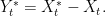
Intriguingly, various constructions related to Brownian motion result in quantities with moments described by the Riemann zeta function. These distributions appear in integral representations used to extend the zeta function to the entire complex plane, as described in an earlier post. Now, I look at how they also arise from processes constructed from Brownian motion such as Brownian bridges, excursions and meanders.
Recall the definition of the Riemann zeta function as an infinite series
 |
which converges for complex argument s with real part greater than one. This has a unique extension to an analytic function on the complex plane outside of a simple pole at s = 1.
Often, it is more convenient to use the Riemann xi function which can be defined as zeta multiplied by a prefactor involving the gamma function,
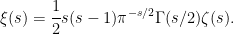 |
This is an entire function on the complex plane satisfying the functional equation ξ(1 - s) = ξ(s).
It turns out that ξ describes the moments of a probability distribution, according to which a random variable X is positive with moments
![\displaystyle {\mathbb E}[X^s]=2\xi(s),](https://s0.wp.com/latex.php?latex=%5Cdisplaystyle++%7B%5Cmathbb+E%7D%5BX%5Es%5D%3D2%5Cxi%28s%29%2C+&bg=ffffff&fg=000000&s=0&c=20201002) |
(1) |
which is well-defined for all complex s. In the post titled The Riemann Zeta Function and Probability Distributions, I denoted this distribution by Ψ, which is a little arbitrary but was the symbol used for its probability density. A related distribution on the positive reals, which we will denote by Φ, is given by the moments
![\displaystyle {\mathbb E}[X^s]=\frac{1-2^{1-s}}{s-1}2\xi(s)](https://s0.wp.com/latex.php?latex=%5Cdisplaystyle++%7B%5Cmathbb+E%7D%5BX%5Es%5D%3D%5Cfrac%7B1-2%5E%7B1-s%7D%7D%7Bs-1%7D2%5Cxi%28s%29+&bg=ffffff&fg=000000&s=0&c=20201002) |
(2) |
which, again, is defined for all complex s.
As standard, complex powers of a positive real x are defined by xs = eslogx, so (1,2) are equivalent to the moment generating functions of logX, which uniquely determines the distributions. The probability densities and cumulative distribution functions can be given, although I will not do that here since they are already explicitly written out in the earlier post. I will write X ∼ Φ or X ∼ Ψ to mean that random variable X has the respective distribution. As we previously explained, these are closely connected:
- If X ∼ Ψ and, independently, Y is uniform on [1, 2], then X/Y ∼ Φ.
- If X, Y ∼ Φ are independent then √X2 + Y2 ∼ Ψ.
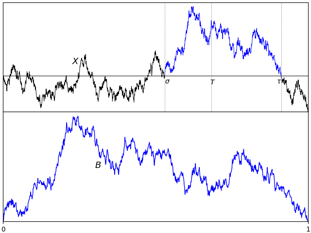
The purpose of this post is to describe some constructions involving Brownian bridges, excursions and meanders which naturally involve the Φ and Ψ distributions.
Theorem 1 The following have distribution Φ:
- √2/πZ where Z = supt|Bt| is the absolute maximum of a standard Brownian bridge B.
- Z/√2π where Z = suptBt is the maximum of a Brownian meander B.
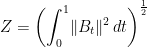
- √2πZ where Z is the sample standard deviation of a Brownian bridge B,
with sample mean B̅ = ∫01Bt dt.
- √π/2Z where Z is the pathwise Euclidean norm of a 2-dimensional Brownian bridge B = (B1, B2),
- √τπ/2 where τ = inf{t ≥ 0: ‖Bt‖= 1} is the first time at which the norm of a 3-dimensional standard Brownian motion B = (B1, B2, B3) hits 1.

The Kolmogorov distribution is, by definition, the absolute maximum of a Brownian bridge. So, the first statement of theorem 1 is saying that Φ is just the Kolmogorov distribution scaled by the constant factor √2/π. Moving on to Ψ;
Theorem 2 The following have distribution Ψ:
- √2/πZ where Z = suptBt – inftBt is the range of a standard Brownian bridge B.
- √2/πZ where Z = suptBt is the maximum of a (normalized) Brownian excursion B.
- √π/2Z where Z is the pathwise Euclidean norm of a 4-dimensional Brownian bridge B = (B1, B2, B3, B4),

Continue reading “Brownian Motion and the Riemann Zeta Function”


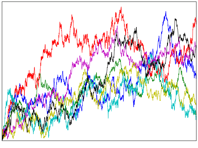


![{[0,T]}](https://s0.wp.com/latex.php?latex=%7B%5B0%2CT%5D%7D&bg=ffffff&fg=000000&s=0&c=20201002) is continuous and equal to zero at both endpoints, we can consider extending to the entire real line by partitioning the real numbers into intervals of length T and replicating the path of the process across each of these. This will result in continuous and periodic sample paths, suggesting another method of representing Brownian bridges. That is, by Fourier expansion. As we will see, the Fourier coefficients turn out to be independent normal random variables, giving a useful alternative method of constructing a Brownian bridge.
is continuous and equal to zero at both endpoints, we can consider extending to the entire real line by partitioning the real numbers into intervals of length T and replicating the path of the process across each of these. This will result in continuous and periodic sample paths, suggesting another method of representing Brownian bridges. That is, by Fourier expansion. As we will see, the Fourier coefficients turn out to be independent normal random variables, giving a useful alternative method of constructing a Brownian bridge.![{[0,1]}](https://s0.wp.com/latex.php?latex=%7B%5B0%2C1%5D%7D&bg=ffffff&fg=000000&s=0&c=20201002) . This does not reduce the generality, since bridges on an interval
. This does not reduce the generality, since bridges on an interval 
 , where
  is an IID sequence of standard normals. This series converges uniformly in t, both with probability one and in the
  norm for all
  .
. 
 be a fixed time. Then, the process
 is independent from
  .
.  , we just need to show that
 ![{{\mathbb E}[B_sX_t]}](https://s0.wp.com/latex.php?latex=%7B%7B%5Cmathbb+E%7D%5BB_sX_t%5D%7D&bg=ffffff&fg=000000&s=0&c=20201002) is zero. Using the covariance structure
is zero. Using the covariance structure ![{{\mathbb E}[X_sX_t]=s\wedge t}](https://s0.wp.com/latex.php?latex=%7B%7B%5Cmathbb+E%7D%5BX_sX_t%5D%3Ds%5Cwedge+t%7D&bg=ffffff&fg=000000&s=0&c=20201002) we obtain,
we obtain,![\displaystyle {\mathbb E}[B_sX_t]={\mathbb E}[X_sX_t]-\frac sT{\mathbb E}[X_TX_t]=s-\frac sTT=0](https://s0.wp.com/latex.php?latex=%5Cdisplaystyle++%7B%5Cmathbb+E%7D%5BB_sX_t%5D%3D%7B%5Cmathbb+E%7D%5BX_sX_t%5D-%5Cfrac+sT%7B%5Cmathbb+E%7D%5BX_TX_t%5D%3Ds-%5Cfrac+sTT%3D0+&bg=ffffff&fg=000000&s=0&c=20201002)
![{\{B_t\}_{t\in[0,T]}}](https://s0.wp.com/latex.php?latex=%7B%5C%7BB_t%5C%7D_%7Bt%5Cin%5B0%2CT%5D%7D%7D&bg=ffffff&fg=000000&s=0&c=20201002) is a Brownian bridge on the interval
is a Brownian bridge on the interval  for a standard Brownian motion X.
 , then B is called a standard Brownian bridge.
  . See lemma